In this blog post, we will take a deep dive into the OSPF Shortest Path First (SPF) algorithm. We will use a sample topology with asymmetric costs to understand how OSPF calculates the shortest path to all other routers.
Our Topology
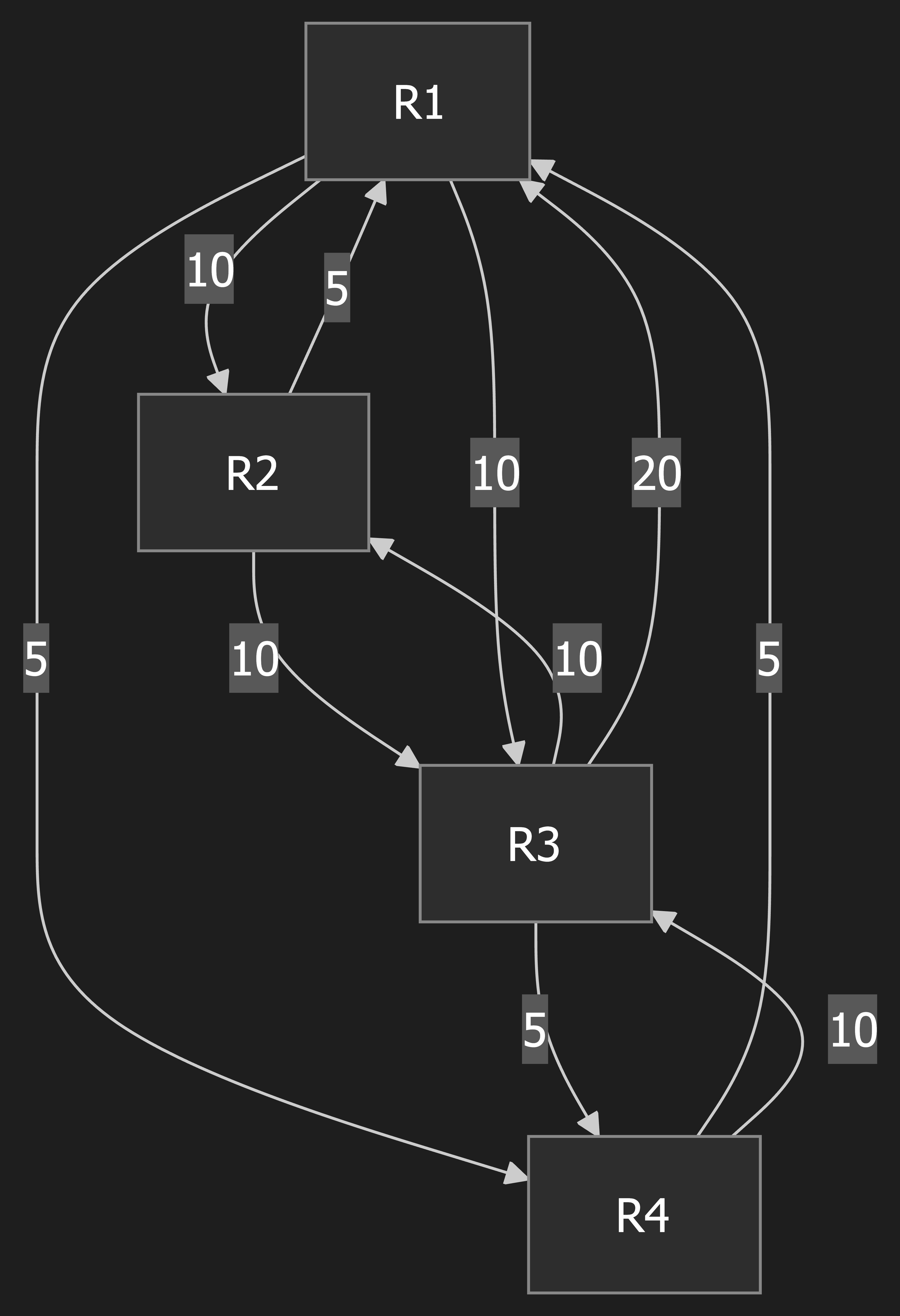
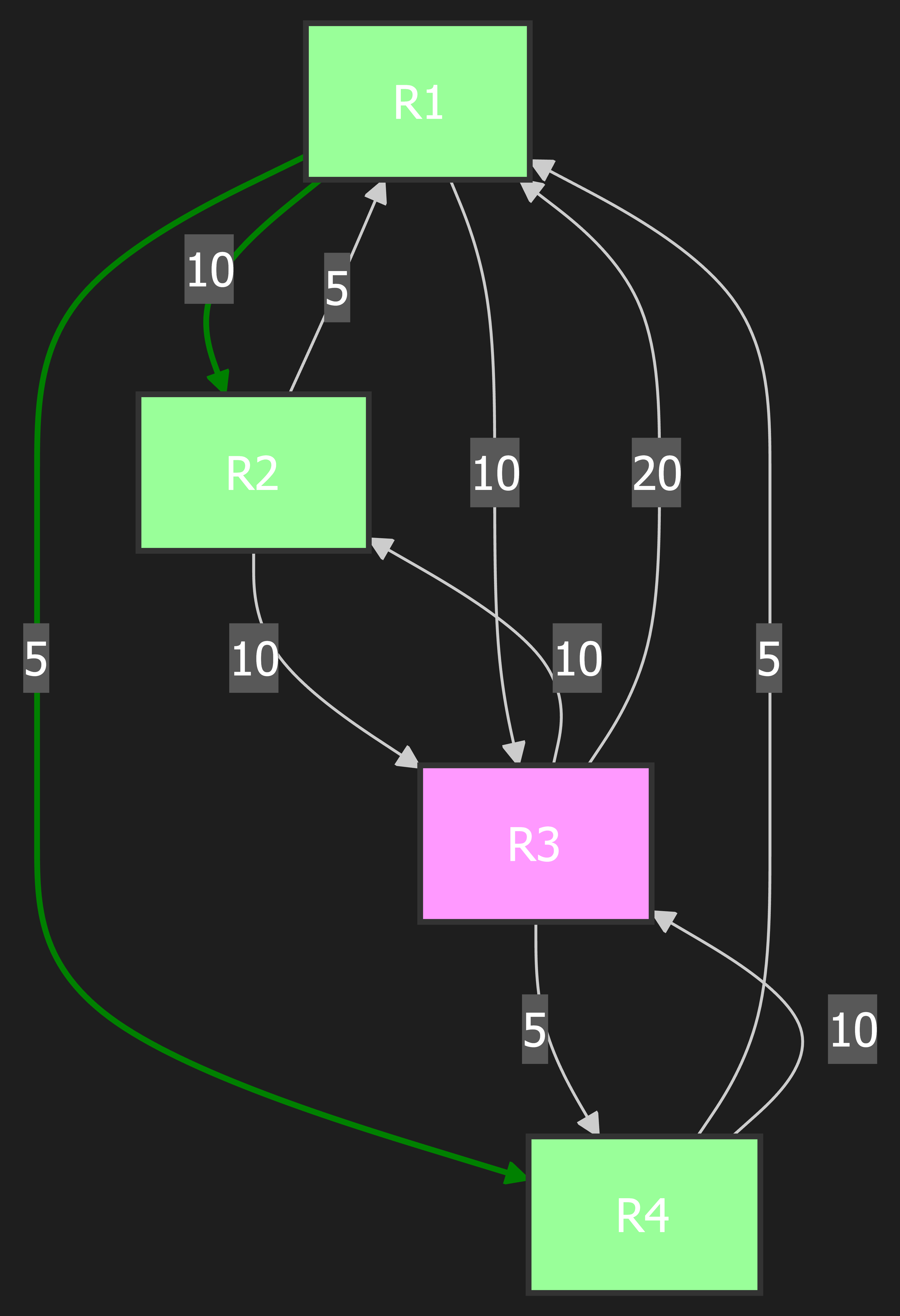
R1 -> R2: 10,R2 -> R1: 5R2 -> R3: 10,R3 -> R2: 10 (Symmetric)R1 -> R4: 5,R4 -> R1: 5 (Symmetric)R4 -> R3: 10,R3 -> R4: 5R1 -> R3: 10,R3 -> R1: 20
We will perform the SPF calculation from the perspective of R1.
Link-State Database (LSDB)
The LSDB stores the LSAs from all routers. With asymmetric costs, the database reflects the cost in the direction advertised by the router.
| Advertising Router | Neighbor | Cost |
|---|---|---|
| R1 | R2 | 10 |
| R1 | R4 | 5 |
| R1 | R3 | 10 |
| R2 | R1 | 5 |
| R2 | R3 | 10 |
| R3 | R2 | 10 |
| R3 | R4 | 5 |
| R3 | R1 | 20 |
| R4 | R1 | 5 |
| R4 | R3 | 10 |
SPF Calculation for R1
Now, let’s perform the SPF calculation from R1’s perspective. We will use two lists: CANDIDATE and PATH.
- PATH: Nodes in the shortest-path tree (Green).
- CANDIDATE: Nodes to be visited (Yellow).
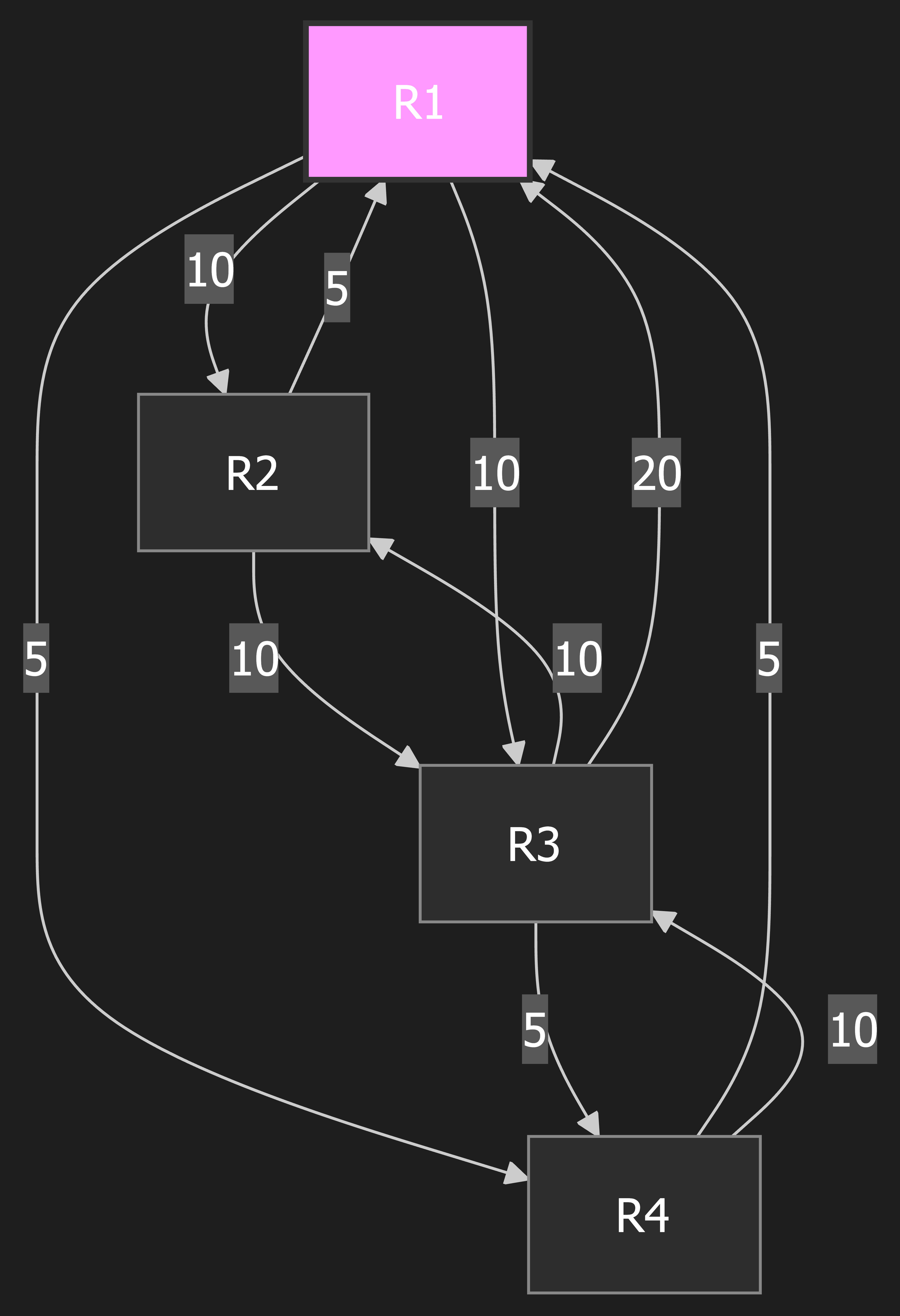
Step 0: Initialization
Explanation: The process begins by setting up our starting point. We place our own router, R1, into the CANDIDATE list. The cost to reach ourselves is always 0. The PATH list is empty because we haven’t calculated any shortest paths yet.
PATH List
| Node | Next Hop | Total Cost |
|---|---|---|
CANDIDATE List
| Node | Next Hop | Total Cost |
|---|---|---|
| R1 | R1 | 0 |
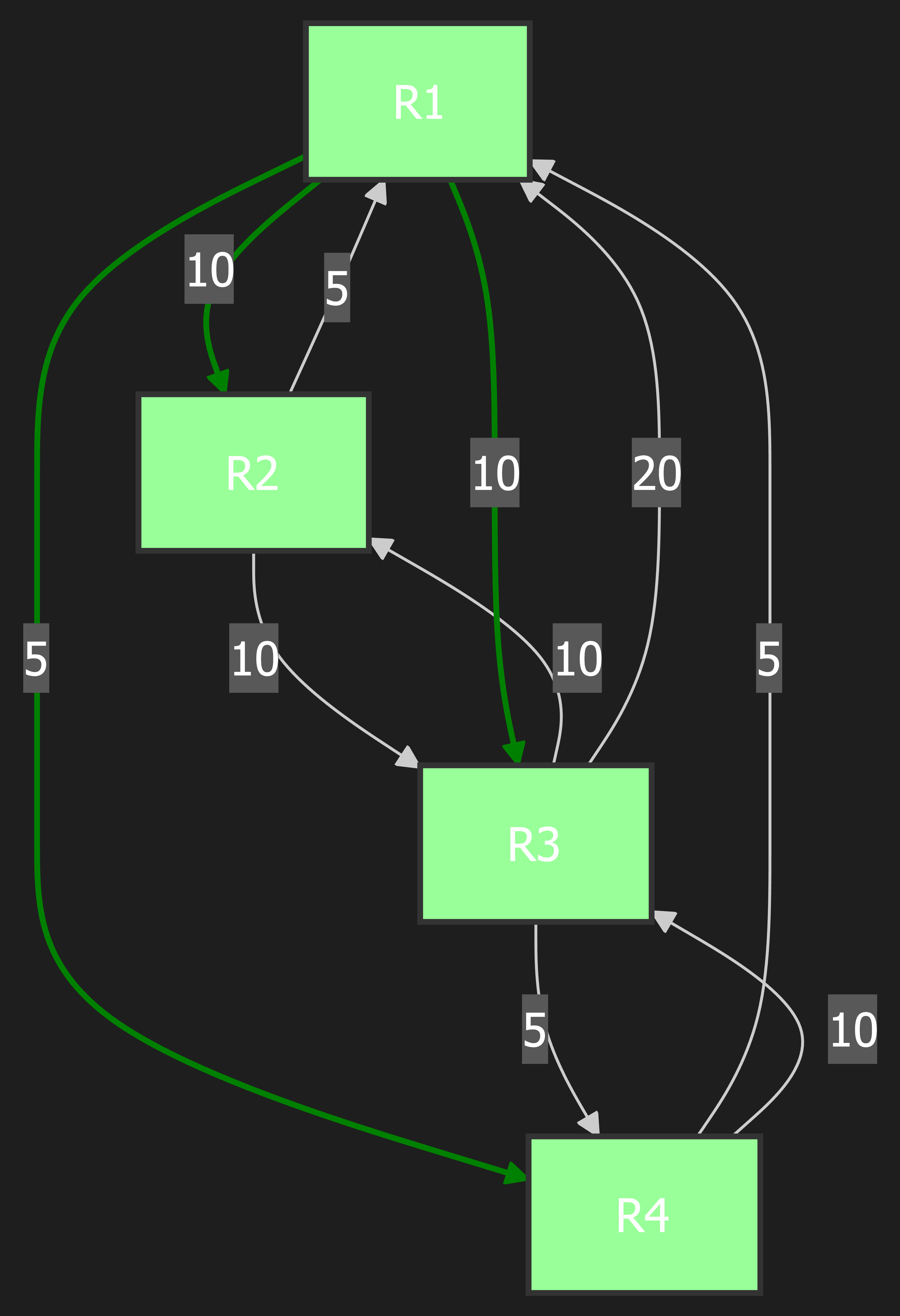
Step 1: Move R1 to PATH
Explanation: We look at the CANDIDATE list and find the node with the lowest cost. Right now, that’s R1 (cost 0). We move R1 to the PATH list, which means we have finalized the shortest path to R1 (it’s ourselves). Now, we look at all of R1’s direct neighbors (R2, R3, and R4) and add them to the CANDIDATE list. Their costs are simply the costs of the direct links from R1.
PATH List
| Node | Next Hop | Total Cost |
|---|---|---|
| R1 | R1 | 0 |
CANDIDATE List
| Node | Next Hop | Total Cost |
|---|---|---|
| R4 | R4 | 5 |
| R2 | R2 | 10 |
| R3 | R3 | 10 |
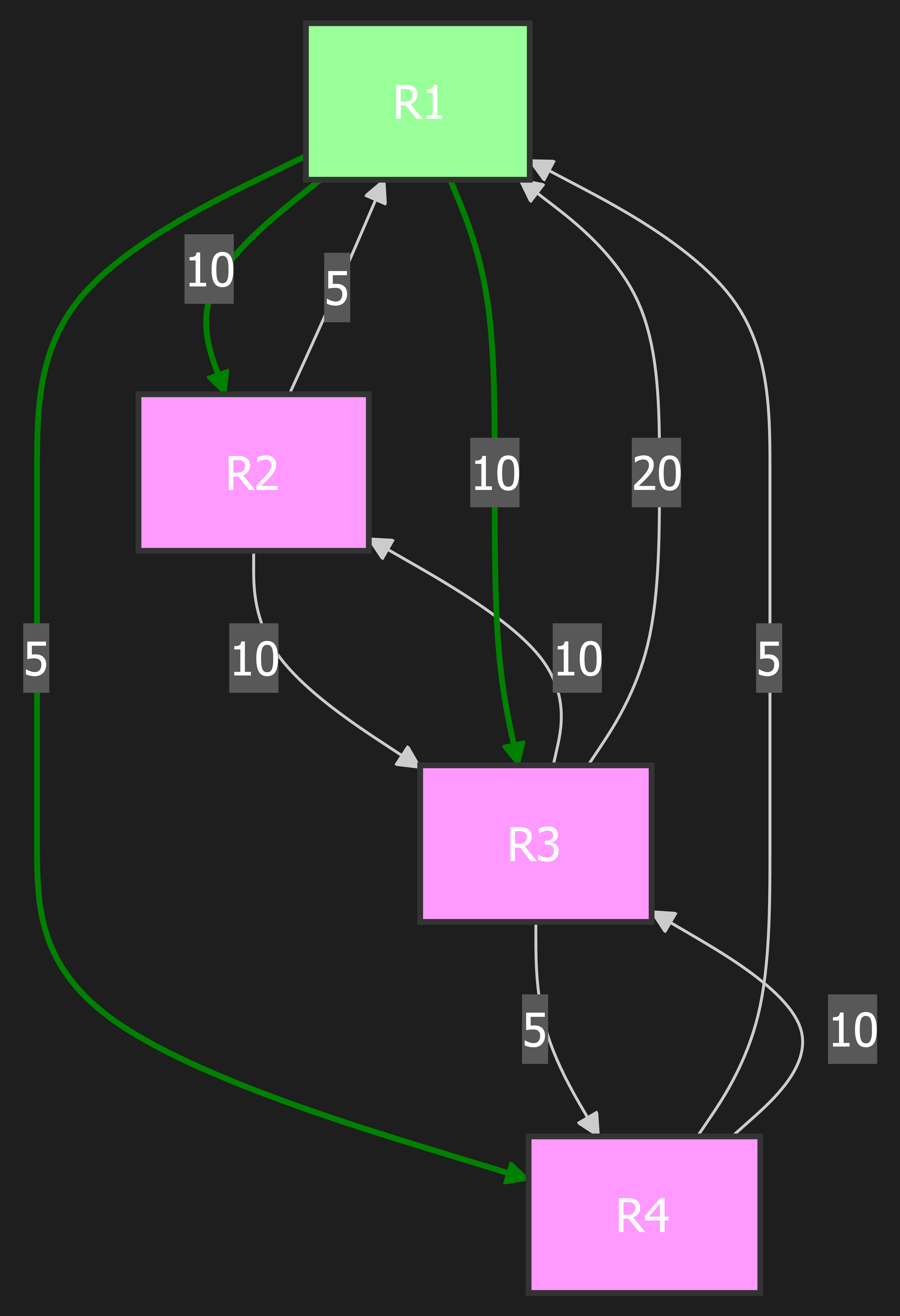
Step 2: Move R4 to PATH
Explanation: We again look for the node with the lowest cost in the CANDIDATE list. R4 has a cost of 5, while R2 and R3 both have a cost of 10. So, we choose R4. We move R4 to the PATH list, finalizing the shortest path to R4. Now, we check R4’s neighbors. R1 is already in the PATH list, so we ignore it. The other neighbor is R3. We calculate the total cost to reach R3 through R4: (Cost to R4) + (Cost from R4 to R3) = 5 + 10 = 15. We then check if there’s already an entry for R3 in the CANDIDATE list. There is, and its cost is 10. Since our new calculated cost (15) is higher than the existing cost (10), we do nothing. We always keep the lower-cost path.
PATH List
| Node | Next Hop | Total Cost |
|---|---|---|
| R1 | R1 | 0 |
| R4 | R4 | 5 |
CANDIDATE List
| Node | Next Hop | Total Cost |
|---|---|---|
| R2 | R2 | 10 |
| R3 | R3 | 10 |
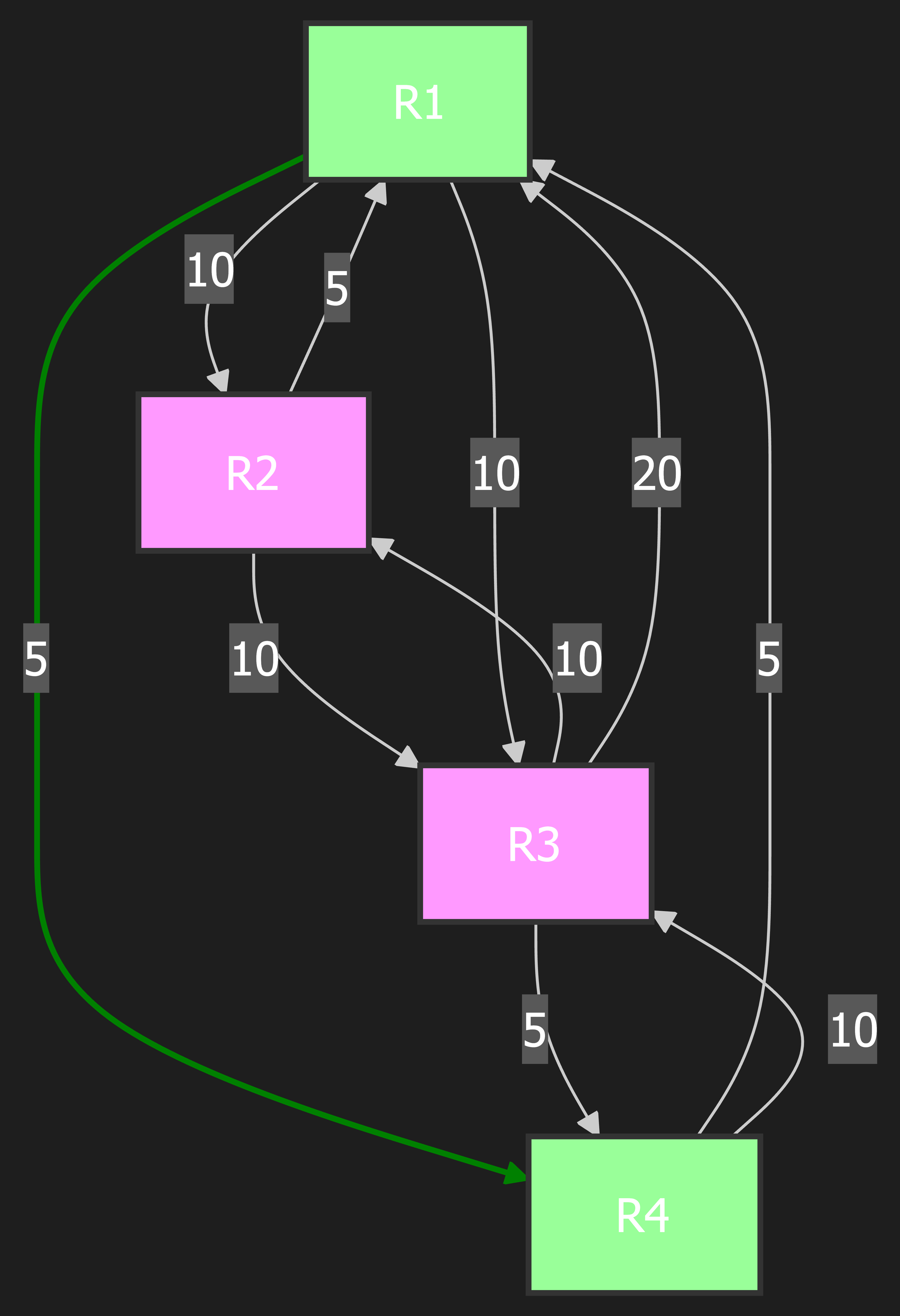
Step 3: Move R2 to PATH
Explanation: Looking at the CANDIDATE list, we have a tie between R2 and R3, both with a cost of 10. The router will pick one (the choice can depend on implementation details, but the outcome will be the same). Let’s say it picks R2. We move R2 to the PATH list. Now, we check R2’s neighbors. R1 is already in PATH. The other neighbor is R3. We calculate the total cost to R3 via R2: (Cost to R2) + (Cost from R2 to R3) = 10 + 10 = 20. We check the CANDIDATE list and see the existing path to R3 has a cost of 10. Since our new cost (20) is higher, we again do nothing.
PATH List
| Node | Next Hop | Total Cost |
|---|---|---|
| R1 | R1 | 0 |
| R4 | R4 | 5 |
| R2 | R2 | 10 |
CANDIDATE List
| Node | Next Hop | Total Cost |
|---|---|---|
| R3 | R3 | 10 |
Step 4: Move R3 to PATH
Explanation: The only node left in the CANDIDATE list is R3. We move it to the PATH list. All of R3’s neighbors (R1, R2, R4) are already in the PATH list, so there are no new paths to consider. The CANDIDATE list is now empty, which signals that the algorithm is finished. We have found the shortest path to every router in the network.
PATH List
| Node | Next Hop | Total Cost |
|---|---|---|
| R1 | R1 | 0 |
| R4 | R4 | 5 |
| R2 | R2 | 10 |
| R3 | R3 | 10 |
CANDIDATE List
| Node | Next Hop | Total Cost |
|---|---|---|
The CANDIDATE list is empty. The algorithm is complete.
Shortest Path Tree (SPT) for R1
The final PATH list gives us the Shortest Path Tree from R1’s perspective.
| Destination | Next Hop | Total Cost |
|---|---|---|
| R1 | Self | 0 |
| R2 | R2 | 10 |
| R3 | R3 | 10 |
| R4 | R4 | 5 |
R1’s Routing Table
Based on the SPT, here is the final routing table for R1.
| Destination | Next Hop | Cost |
|---|---|---|
| R2 | R2 | 10 |
| R3 | R3 | 10 |
| R4 | R4 | 5 |